")
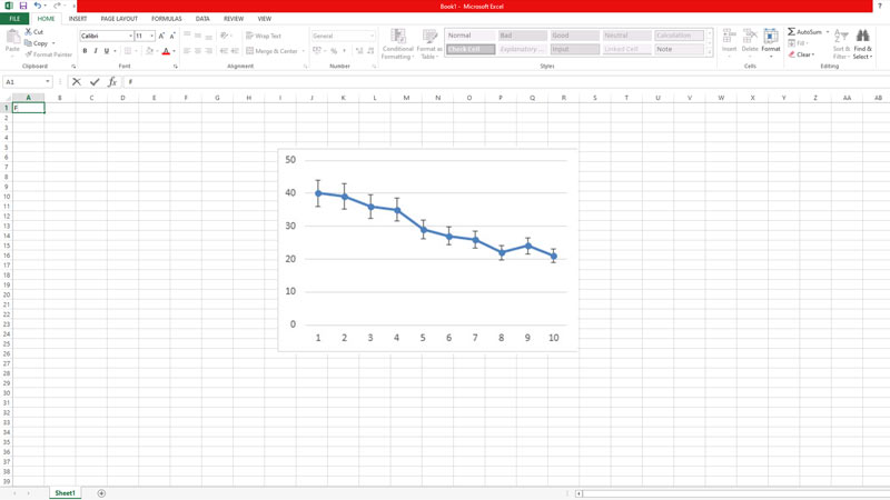
While using the charts for professional purposes on Excel sheets a user might prefer to use the error bars to represent the margin of errors and Standard Deviations. Fortunately, Microsoft Excel provides the flexibility to add error bars to your charts. You can add them to all the data points in the data series of your charts, and you can learn to use them with the help of this guide.
Microsoft Excel: How to Add Error Bars (2023)
On your Windows or Mac computers, you can add Error bars on your Excel chart to show the margin of errors or standard deviation by following the below-mentioned workaround:
1. Add Error Bars on Windows
- First create a 2-D area, bar, column, line, XY (scatter), or bubble chart on your Excel app.
- Then, click anywhere on the chart and select the ‘+’ button.
- The Chart elements menu will open.
- Tick the ‘Error Bars’ checkbox by clicking on it.
- To change the error amount, click the arrow next to the ‘Error Bars’ and select any one type from the given default options (Standard Error, Percentage, or Standard Deviation).
- Also, you can customize the error amount by selecting ‘More Options’ from the list and choosing the options under the ‘Vertical Error Bar’ or ‘Horizontal Error Bar’ sections.
2. Add Error Bars on Mac
- Click the chart data series in the chart i.e., if it’s a line chart, click the line, if it’s a bar graph, click on bars to select them.
- Once you select the data series, click the ‘Add Chart Element’ button on the ‘Chart Design’ tab.
- Now select the Error Bars and select any one of the default options i.e., Standard Error, Percentage, or Standard Deviation.
- If you want a custom error amount, click the ‘More Error Bars Options’ from the menu.
- Then, click ‘Custom’ under the ‘Error Amount’ section.
- Finally, click the ‘Specify Value’ button and enter the Positive Error Value and Negative Error Value under their respective fields and click the ‘OK’ button to save changes.
That’s everything covered on how to add error bars in Excel. Also, check out our other guides, such as How to add a Checkbox in Microsoft Excel or How to freeze rows and columns on Microsoft Excel on your Windows 10 desktop.