To make your Excel spreadsheet more readable and visually appealing, you might want to highlight every other row with a different color. This is also known as zebra striping or alternating row colors. Highlighting rows can be helpful as they help identify cells more comfortably and there are a few tools in Excel to help you do it. Hence, to color the rows in Excel, this guide will help you.
Excel: How to Highlight Every Other Row (2023)
To highlight every other row in Excel, you can use the Conditional Formatting feature, and here’s how you can do it:
- Firstly, select the range of cells to which you want to apply the formatting.
- Then, open the ‘Conditional Formatting’ menu from the ‘Home’ tab.
- Now click the ‘New Rule’ option, and select the ‘Use a formula to determine which cells to format’ option.
- In the ‘New Formatting Rule’ dialog box, enter the following formula in the ‘Format values where this formula is true’ box:
=MOD(ROW(),2)=0
- This formula checks if the row number is divisible by 2, and returns ‘TRUE’ for even rows and ‘FALSE’ for odd rows.
- Then, click the ‘Format’ button and go to the ‘Fill’ tab.
- Now select the color for the even rows.
- Also, you can change other formatting options such as font, border, or number format by going to different tabs.
- Click the ‘OK’ button to close the ‘Format Cells’ dialog box.
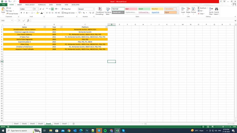
- Finally, click the ‘OK’ button again to apply the conditional formatting rule to your selected range.
- Now you should see every other row highlighted with the color you chose.
Highlight Odd rows
- Using Conditional Formatting you can choose to highlight odd rows by following these steps:
- Firstly, open the ‘New Formatting Rule’ dialogue box from the ‘Conditional Formatting’ menu from the above-mentioned steps:
- Then type the following formula in the ‘Format values where this formula is true’ box:
=MOD(ROW(),2)=1
- Now click the ‘Format’ button and go to the ‘Fill’ tab.
- Finally, select a different fill color for the odd rows and click the ‘OK’ button to apply changes.
That’s everything covered on how to highlight every other row in Excel. Also, check out our other guides, such as How to remove empty/blank rows in Excel or How to unhide rows in Excel.