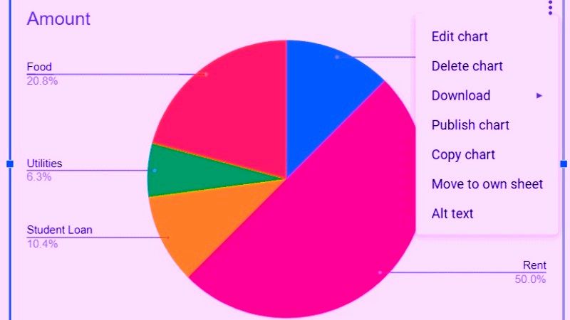
Google Sheets is an online web app that allows users to do a lot of things such as creating, editing, and sharing single sheets or spreadsheets online. Besides that, it’s a convenient solution for creating pie charts. In this article, we’ll walk you through on how to create Pie Chart in Google Sheets in the easy steps below.
Google Sheets: How to Create a Pie Chart (2023)

The first thing you will need to do is register a Google account or log into your own Gmail account, if you already have one. Once that’s done, follow the instructions below to add a pie chart to a spreadsheet using Google Sheets.
- First, launch the Google Sheets in a browser such as Google Chrome and create a new spreadsheet.
- After that, type or copy-paste your data into the Google worksheet, select it (including titles), and click Insert > Chart to open the Chart Editor.
- From the available menu, select the type of pie chart you prefer. By doing so, a pie chart generated by Google Sheets based on the data entered will appear on your spreadsheet.
- If you want to customize the pie chart with Google Sheets, click the Customize tab in the Chart Editor panel. So you can change the style of the chart, alter the colors, add or remove titles and wordings, and more.
- Now you need to click on the 3 vertical dots icon at the top right of the graph pane and select Edit Graph to reopen Graph Editor. Google Sheets also allows you to delete, download, publish, copy, or move pie charts and any other diagrams.
- That’s it, in this way, you have now created a pie chart in Google Sheets.
That is all you need to know about how to create or make a pie chart in Google Sheets. For more Google Sheets Tips and Tricks, check out our other guides only on our website TechNClub.com: How to Password Protect Google Sheets, and How to Identify Duplicates in Google Sheets.
