If you have ever worked with a large spreadsheet in Excel, you may have encountered the problem of hidden rows. Sometimes, you may want to hide some rows to make your data more compact or to focus on a specific subset of information. However, you may also want to unhide those rows later to see the full picture or to make changes to the data. There are a few ways to unhide rows in Excel, and this guide will help you with it.
Excel: How to Unhide Rows (2023)
You can unhide rows on your Excel sheet, using the Home tab, or from the context menu, and here’s how you can do it:
1. From the Home Tab

Using the Home tab to unhide rows is useful when you want to unhide rows under a specific range. Also, you can unhide all the rows at once using this method, and you can do this by following these steps:
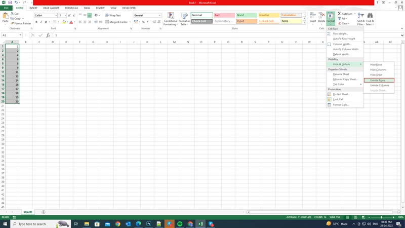
- Firstly, select the rows above and below the hidden rows. For example, if you have hidden row 5, select rows 4 and 6.
- Then go to the ‘Home’ tab and click the ‘Format’ icon from the ‘Cells’ group.
- Now select the ‘Hide & Unhide’ option under the ‘Visibility’ section.
- Finally, click the ‘Hide Rows’ option from the new sub-menu.
- This will unhide all the hidden rows in the selected range.
2. Use Context Menu

Another way to unhide rows in Excel is to use the context menu. This method works if you know the exact row numbers of the hidden rows, and you want to unhide them individually. Hence, to unhide rows using the Go-To dialog box, follow these steps:
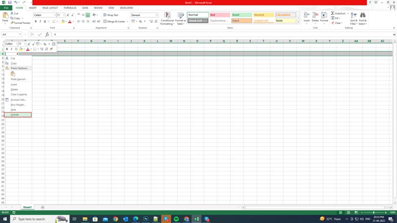
- Firstly, hover the cursor over the space between two-row numbers and right-click on it. For example, if Row 5 is hidden, right-click on the space between rows 4 and 6.
- This will open the context menu.
- Finally, select the ‘Unhide’ option from the menu and the hidden row will become visible.
That’s everything covered on how to unhide rows in Excel. Also, check out our other guides, such as How to separate names in Excel or How to use DATEDIF in Excel.
